2D Grid with factors and conductances

This example illustrates how to setup and run a 2D grid simulation, using options to modify conductances and parameters for each cell. For this example we will setup a grid with a non-conducting center.

Setup & Run the Simulation

First we will setup the simulation so that the border cells are all conducting cells while the internal cells are not excitable, creating a ring of excitable cells

import PyLongQt as pylqt
import numpy as np
import pandas as pd
import matplotlib.pyplot as plt

proto = pylqt.protoMap['Grid Protocol']()

n_cols = 5
n_rows = 5

proto.grid.addRows(n_rows)
proto.grid.addColumns(n_cols)

border_cells = {(i,0) for i in range(n_rows)} | \
    {(0,i) for i in range(n_cols)} | \
    {(i,4) for i in range(n_rows)} | \
    {(4,i) for i in range(n_cols)}

for row,col in border_cells:
    node = proto.grid[row,col]
    node.setCellByName('Canine Ventricular (Hund-Rudy 2009)')

proto.grid.simpleGrid()

Out:

(array([[0, 0, 0, 0, 0],
       [0, 1, 1, 1, 0],
       [0, 1, 1, 1, 0],
       [0, 1, 1, 1, 0],
       [0, 0, 0, 0, 0]]), {'Canine Ventricular (Hund-Rudy 2009)': 0, 'Inexcitable Cell': 1})

Lets only stimulate the middle cell in the 1st column

proto.stimNodes = {(2,0)}

proto.stimt = 1000
proto.stimval = -150

And add some measures for each of the excitable cells

proto.measureMgr.dataNodes = border_cells

proto.measureMgr.addMeasure('vOld', {'peak', 'min', 'cl'})
proto.measureMgr.addMeasure('iNa', {'min', 'avg'})
proto.measureMgr.selection

Out:

{'iNa': {'min', 'avg'}, 'vOld': {'min', 'peak', 'cl'}}

and some traces

proto.cell.variableSelection = {'t', 'vOld', 'iNa'}

There are a few further customizations which we will show for the grid (they are also available for a fiber). The first is the cell constants (called pvars, such as the Factors used in the parameter sensitivity analysis example) which allow for values of the parameters to be set. Unlike for the single cell, the parameters are not for running multiple simulations, rather they are for the spatial positioning of the parameter values across the grid.

proto.pvars['InaFactor'] = proto.pvars.IonChanParam(proto.pvars.Distribution.none, 1, -0.05)
proto.pvars.setStartCells('InaFactor', {(0,3)})
proto.pvars.setMaxDistAndVal('InaFactor', 2, 1)

The first line above adds a rule for the sodium current. The first argument is the starting value and the second is how much the value should decrease for each node of distance it moves away from the starting cell. The starting cell has not yet been set and the default behavior is for every cell to be a start cell. To fix this we set a single start cell on the next line using the setStartCells() method.

We can also set limitations on the cells that will be effected, by limiting the maximum distance at which the rule will be applied, and the maximum value that the rule will apply. These are the first and second arguments of the next line restricting the distance to two steps away, and not changing the maximum value.

Now lets create a small visualization of how all these rules will be applied

vis = np.ones(proto.grid.shape)
cells_list = list(proto.pvars['InaFactor'].cells.keys())
idx_list = tuple(zip(*cells_list))
vis[idx_list] = list(proto.pvars['InaFactor'].cells.values())
vis

Out:

array([[1.  , 0.9 , 0.95, 1.  , 0.95],
       [1.  , 1.  , 1.  , 1.  , 0.9 ],
       [1.  , 1.  , 1.  , 1.  , 1.  ],
       [1.  , 1.  , 1.  , 1.  , 1.  ],
       [1.  , 1.  , 1.  , 1.  , 1.  ]])

Notice that the rule is not being applied to the inexcitable cells. This is because PyLongQt checks whether each cell has the ion channel constant and only applies the rule to those cells.

Note

The pvars settings can also be used to apply arbitrary values to the cells during the setup process by manually changing proto.pvars[‘InaFactor’].cells. In this case the rules may indicate that a change will be applied to a cell, which doesn’t have that ion channel. That assignment will be ignored when the simulation is being run.

The other optional configuration is to change the conductances between cells. Setting conductances to smaller values will reduce the influence of cells on their neighbor, while setting them to larger values will do the oppisite. Choosing to set a conductance to 0 will completely remove any effect of those two cells on each other. Conductances are also symmetric, so a cell’s right side conductance is its right-hand neighbors left conductance. When setting conductances this will be updated automatically. Conductances on the boarder of the Grid will always be 0, and cannot be changed. Similarly, inexcitable cells will always have a conductance of 0 with all of their neighbors. For this example we will reduce the conductance between the nodes on the top and bottom of our ring of cells. One way to accomplish this is to set the conductivitiy value directly using Node.setConductivityDirect(). This is a direct method as the value is set given the provided value regardless of the cell’s properties. Another way to change the conductance is to set the resistivity using Node.setResistivity(). Using this method, we change the gap junction resistance by a percentage which will impact the conductivity while still using a physiological calculation.

for i in range(proto.grid.columnCount()):
    node = proto.grid[0,i]
    node.setResistivity(pylqt.right, percentage=120)

Now the simulation is all setup and can be run.

sim_runner = pylqt.RunSim()
sim_runner.setSims(proto)
sim_runner.run()
sim_runner.wait()

Plot the Results

Disable future warnings to avoid excess outputs from plotting

import warnings
warnings.simplefilter(action='ignore', category=FutureWarning)

The data can once again be read using DataReader.

[trace], [meas] = pylqt.DataReader.readAsDataFrame(proto.datadir)

Then we will calculate the distance from the simulus for each border cell

dists = dict()
stim_cell = np.array((2,0))
for cell in border_cells:
    diff = np.array(cell) - stim_cell
    dist = np.sum(np.abs(diff))
    dists[cell] = dist

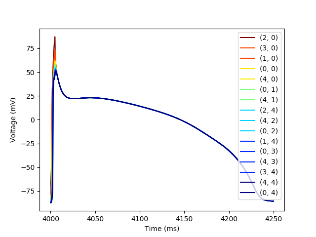
We can use the trace Dataframe to produce traces of each of the action potenitals in the fiber and color them by their location in the fiber

plt.figure()
colors = plt.cm.jet_r(np.linspace(0,1,max(dists.values())+1))
for cell in sorted(border_cells, key=lambda x: dists[x]):
    trace_subset = trace[trace[(cell,'t')] < 4_250]
    plt.plot(trace_subset[(cell,'t')],
             trace_subset[(cell,'vOld')],
             color=colors[dists[cell]],
             label=str(cell))
plt.xlabel('Time (ms)')
plt.ylabel('Voltage (mV)')
_ = plt.legend()

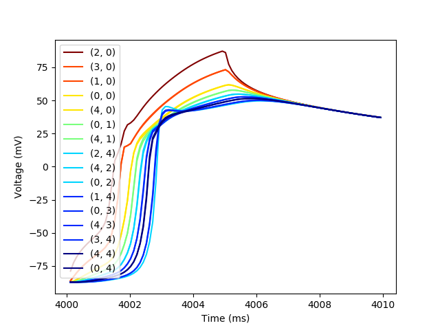
Then let’s create one more plot to show the action potential propagation.

plt.figure()
colors = plt.cm.jet_r(np.linspace(0,1,max(dists.values())+1))
for cell in sorted(border_cells, key=lambda x: dists[x]):
    trace_subset = trace[trace[(cell,'t')] < 4_010]
    plt.plot(trace_subset[(cell,'t')],
             trace_subset[(cell,'vOld')],
             color=colors[dists[cell]],
             label=str(cell))
plt.xlabel('Time (ms)')
plt.ylabel('Voltage (mV)')
_ = plt.legend()