Parameter Sensitivity Analysis

This example illustrates how to conduct parameter sensitivity analysis. The purpose of conducing this kind of analysis is to determine the impact of one (or more) cell parameter, such as sodium ion channel conductance, on one (or more) measurable output, such as upstroke velocity. For this example we will stick to one cell parameter and one output, however the technique is not changed when preforming this analysis for many inputs possible outputs, except that a larger number of simulations may be required. The approach of this analysis can be divided into 3 parts:

1. Generate a population of cells. The cells in this population are not all the same and instead vary randomly with respect to the parameters of interest. Typically they are generated from a normal or lognormal distribution, who’s spread is tuned to cover a reasonable range of possible inputs. The definition of a reasonable range depends on the purpose of the analysis, for example if the goal is to understand the parameter’s effect in healthy cells, then the population generated should correspond to a range of plausible values for healthy cells.

2. Run a simulation for each cell in the generated population and measure the resulting outputs.

3. Conduct a linear regression using the parameters as predictors and the measured output as the response. This creates a linear model who’s coefficients indicated the effect of a change in a parameter to a change in response.

For this example we will specifically be looking at the effect of sodium channel conductance on upstroke velocity.

import PyLongQt as pylqt

import pandas as pd

Setup the Simulation & Configure the population

The initial setup is the same as before

proto = pylqt.protoMap['Current Clamp Protocol']()

proto.setCellByName('Canine Ventricular (Hund-Rudy 2009)')

proto.bcl = 800
proto.tMax = 50_000
proto.numstims = 200
proto.meastime = 1_000
proto.writetime = 51_000 #We do not need to write any traces!

proto.cell.variableSelection = set()

proto.measureMgr.percrepol = 90
proto.measureMgr.addMeasure('vOld', {'peak', 'maxderiv'})

The new addition beyond the ‘simple current clamp’ example is the use of Protocol.pvars to modify the sodium channel conductance for each simulation.

To get a list of the possible parameters use Cell.pars

list(proto.cell.pars.keys())[:5]

Out:

['AGeo', 'Rcg', 'FDAY', 'InacaFactorbulk', 'Ito2Factor']

Parameter names that end in Factor scale the parameter, so that 1 is the default value for all factors, and their reasonable range is 0 to infinity.

The factor we need is InaFactor, and to set up the pvars entry we need to specify the distribution that will be used to generate the values we will use lognormal, so we will also need to specify the mean and standard deviation of that distribution.

distribution = proto.pvars.Distribution.lognormal
mean = 0
st_dev = 0.2

proto.pvars['InaFactor'] = proto.pvars.IonChanParam(distribution, mean, st_dev)

proto.pvars['InaFactor']

Out:

<TIonChanParam: Lognormal Distribution (Mean: 0.000000 Standard Deviation: 0.200000)>

Finally we need to specify the number of simulations to generate from the popultion. We will generate 20 in this case, although 300-600 is a more typical number.

proto.numtrials = 20

As an aside, the specific values for each trial are stored in Protocol.pvars and can be viewed (or modified!), below are the first 5 values

proto.pvars['InaFactor'].trials[:5]

Out:

[1.534903253124452, 0.7789928077395771, 1.0263547171177279, 1.2129733201298847, 0.9115086295274883]

Run the simulations

The simulation can be run using the exact same syntax as before. RunSim automatically detects the number of trails to be run and handles them concurrently.

sim_runner = pylqt.RunSim()
sim_runner.setSims(proto)
sim_runner.run()
sim_runner.wait()

Read the data & fit linear regression model

Reading the data is preformed similarly, however the lists returned now have 20 elements instead of 1, with each DataFrame being for one simulation.

traces, meases = pylqt.DataReader.readAsDataFrame(proto.datadir)

For upstroke velocity we are interested in the final action potential for each simulation rather than all the values, so we will compile that into its own DataFrame first

last_meas = pd.DataFrame([
    meas
    .loc[meas.index[-1]]
    .rename(i)
    for i,meas in enumerate(meases)])

A detailed explanation for those unfamiliar with python classes

To unpack a little about how this line of code works, it uses a generator expression […] to generate a list of series which pandas then compiles back into a dataframe. More specifically, for i,meas in enumerate(meases) gets each individual measure (which we name meas) dataframe from the meases list and enumerates them, 1…20, which we name i. Then, we get the last row from each meas, using meas.loc[meas.index[-1]]. Finally, we need to rename the Pandas.Series (the row from the dataframe) so that it will have the correct index when they are all compiled into a new dataframe (last_meas), without this last step, all of the rows in the last_meas dataframe would have the same index.

Next we would like to have a copy of the parameter values used in the simulations, which we will get in the same manner as shown earlier.

parameters = pd.Series(proto.pvars['InaFactor'].trials, name='InaFactor')

Now that we have all the data we need we can run a linear regression using the statsmodels pacakge

import statsmodels.api as sm
import seaborn as sns

model = sm.OLS(last_meas[('vOld', 'peak')], sm.add_constant(parameters))
res = model.fit()
print(res.summary())

#%
# The `res` object contains the results of the model fit as well as model
# evaluation criteria, and can be used to determine how much of a change
# in INaFactor will result in a change in upstroke velocity

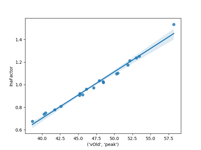
# Finally, as this is a simple linear regression we can generate a plot
# of the points as well as our fit model to examine how strong the model
# looks
_ = sns.regplot(last_meas[('vOld', 'peak')], parameters)

Out:

C:\Users\grat05\AppData\Local\Programs\Python\Python37\lib\importlib\_bootstrap.py:219: RuntimeWarning: numpy.ufunc size changed, may indicate binary incompatibility. Expected 192 from C header, got 216 from PyObject
  return f(*args, **kwds)
                            OLS Regression Results
==============================================================================
Dep. Variable:       ('vOld', 'peak')   R-squared:                       0.983
Model:                            OLS   Adj. R-squared:                  0.982
Method:                 Least Squares   F-statistic:                     1059.
Date:                Mon, 04 Oct 2021   Prob (F-statistic):           1.91e-17
Time:                        16:27:48   Log-Likelihood:                -19.488
No. Observations:                  20   AIC:                             42.98
Df Residuals:                      18   BIC:                             44.97
Df Model:                           1
Covariance Type:            nonrobust
==============================================================================
                 coef    std err          t      P>|t|      [0.025      0.975]
------------------------------------------------------------------------------
const         23.3579      0.753     31.019      0.000      21.776      24.940
InaFactor     23.8657      0.734     32.535      0.000      22.325      25.407
==============================================================================
Omnibus:                        5.869   Durbin-Watson:                   1.368
Prob(Omnibus):                  0.053   Jarque-Bera (JB):                3.579
Skew:                          -0.962   Prob(JB):                        0.167
Kurtosis:                       3.769   Cond. No.                         9.87
==============================================================================

Warnings:
[1] Standard Errors assume that the covariance matrix of the errors is correctly specified.

This model naturally fits quite well. In other scenarios it may be necessary preform a more complete linear regression with model diagnostics, etc to insure model quality. There are many tutorials on linear regression that cover the appropriate steps for running a regression.