3. 1D Grid Simulation

This example illustrates how to setup and run a simple 1D grid simulation, also known as a fiber simulation with a row of cells. These simulations show how the cell models interact rather than examining them in isolation. 2D grids can be setup in the same fashion as 1D fibers, and there is also a more advanced tutorial on setting up a 2D grid showing the possible customizations.

Setup & Run the Simulation

Import PyLongQt and create a grid protocol, this protocol can function for 1 or 2D simulations. These simulations are similar to current clamp simulations except that they are preformed on a grid of connected cells, instead of on an individual cell.

import PyLongQt as pylqt

proto = pylqt.protoMap['Grid Protocol']()

To configure the size of the Fiber we will add one row and the number of columns we would like to have for the simulation. Due to the detailed nature of many of the cell models, larger fibers/grids may be very slow and computationally demanding.

n_cols = 10
proto.grid.addRow()
proto.grid.addColumns(n_cols)

We can also use the Grid.simpleGrid() to get a representation of the grid that is easier to visualize

proto.grid.simpleGrid()

Out:

(array([[0, 0, 0, 0, 0, 0, 0, 0, 0, 0]]), {'Inexcitable Cell': 0})

When new cells are added to the grid, they are automatically filled with a cell model called ‘Inexcitable Cell’, this cell acts like the edge of the grid. It is not excited by its neighbors and cannot pass any signal between them. To replace these cells with more interesting cells, we will create new cell objects and place them in the grid.

To get the possible options for a node in a grid use

proto.grid[0,0].cellOptions()

Out:

['Inexcitable Cell', 'Canine Ventricular (Hund-Rudy 2009)', 'Canine Ventricular Border Zone (Hund-Rudy 2009)', 'Coupled Inexcitable Cell', 'Human Atrial (Courtemanche 1998)', 'Human Atrial (Grandi 2011)', 'Human Atrial (Koivumaki 2011)', 'Human Atrial (Onal 2017)', 'Human Ventricular (Grandi 10)', 'Human Ventricular (Ten Tusscher 2004)', "Human Ventricular Endocardium (O'Hara-Rudy 2011)", "Human Ventricular Epicardium (O'Hara-Rudy 2011)", "Human Ventricular Mid Myocardial (O'Hara-Rudy 2011)", 'Mammalian Ventricular (Faber-Rudy 2000)', 'Mouse Sinus Node (Kharche 2011)', 'Mouse Ventricular (Bondarenko 2004)', 'Rabbit Sinus Node (Kurata 2008)']

rather than

proto.cellOptions()

Out:

['']

as the cell cannot be set at the protocol level when there is a grid structure.

Note

At this time all nodes will have the same options, so it is not necessary to check each node individually.

for col in range(proto.grid.columnCount()):
    node = proto.grid[0,col]
    node.setCellByName('Canine Ventricular (Hund-Rudy 2009)')

proto.grid.simpleGrid()

Out:

(array([[0, 0, 0, 0, 0, 0, 0, 0, 0, 0]]), {'Canine Ventricular (Hund-Rudy 2009)': 0})

Now that all the cells have been setup we can configure the stimulus settings. Many of the settings are the same, however now we must also select the cells that we want to stimulate. Typically this is one edge or one corner of the grid, but it can be any cells as desired.

proto.stimNodes = {(0,0), (0,1)}

To select which cells will be stimulated create a set of tuples with the positions of cells to be stimulated as shown above.

The rest of the settings can be modified in the same fashion as before.

proto.stimt = 1000

By detault the simulation will be 5000 ms

proto.tMax

Out:

5000.0

Measures and traces can also be taken, the setup is largely similar to single cell simulations with the addition of selecting the nodes to be measured. These nodes can be selected using the MeasureManager and are the same nodes used for saving traces and taking measurements. For this example we will selected every node.

proto.measureMgr.dataNodes = {(0,i) for i in range(proto.grid.columnCount())}

proto.measureMgr.addMeasure('vOld', {'peak', 'min', 'cl'})
proto.measureMgr.addMeasure('iNa', {'min', 'avg'})
proto.measureMgr.selection

Out:

{'iNa': {'min', 'avg'}, 'vOld': {'min', 'peak', 'cl'}}

The traces can be set in the same way as before using Protocol.cell

proto.cell.variableSelection = {'t', 'vOld', 'iNa'}

Now the simulation is all setup and can be run.

sim_runner = pylqt.RunSim()
sim_runner.setSims(proto)
sim_runner.run()
sim_runner.wait()

Plot the Results

Disable future warnings to avoid excess outputs from plotting

import warnings
warnings.simplefilter(action='ignore', category=FutureWarning)

The data can once again be read using DataReader.

import pandas as pd
import numpy as np
import matplotlib.pyplot as plt

[trace], [meas] = pylqt.DataReader.readAsDataFrame(proto.datadir)

The trace DataFrame’s columns now have two levels, one for the cell’s position and one for the variable name.

trace.columns[:5]

Out:

MultiIndex([((0, 2),  'iNa'),
            ((0, 2),    't'),
            ((0, 2), 'vOld'),
            ((0, 5),  'iNa'),
            ((0, 5),    't')],
           names=['Cell', 'Variable'])

Similarly the measure DataFrame’s columns have an additional level for the cell’s position

meas.columns[:5]

Out:

MultiIndex([((0, 0),  'iNa',  'avg'),
            ((0, 0),  'iNa',  'min'),
            ((0, 0), 'vOld',   'cl'),
            ((0, 0), 'vOld',  'min'),
            ((0, 0), 'vOld', 'peak')],
           names=['Cell', 'Variable', 'Property'])

We can use the trace Dataframe to produce traces of each of the action potenitals in the fiber and color them by their location in the fiber

plt.figure()
colors = plt.cm.jet_r(np.linspace(0,1,n_cols))
for i in range(n_cols):
    trace_subset = trace[trace[((0,i),'t')] < 4_250]
    plt.plot(trace_subset[((0,i),'t')],
             trace_subset[((0,i),'vOld')],
             color=colors[i],
             label=str(i))
plt.xlabel('Time (ms)')
plt.ylabel('Voltage (mV)')
_ = plt.legend()

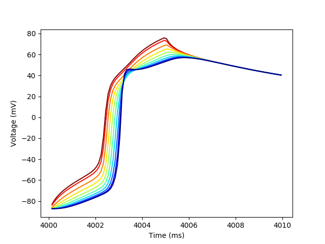
Then let’s create one more plot to show the action potential propagation.

plt.figure()
colors = plt.cm.jet_r(np.linspace(0,1,n_cols))
for i in range(n_cols):
    trace_subset = trace[trace[((0,i),'t')] < 4_010]
    plt.plot(trace_subset[((0,i),'t')],
             trace_subset[((0,i),'vOld')],
             color=colors[i],
             label=str(i))
plt.xlabel('Time (ms)')
_ = plt.ylabel('Voltage (mV)')