1. Simple Current Clamp

This example illustrates how to setup and run a current clamp simulation, also known as a paced simulation on a single cell. Current clamp simulations involve pacing the cell with a set stimulus over time similarly to how the cells would be paced in the heart. To start, once PyLongQt is installed import it as seen below, this gives accesses to all of the classes and objects necessary to set up and run a simulation.

import PyLongQt as pylqt

Setup the Simulation

Protocols are the base of the simulation, the protoMap allows them to be created using their name. Additionally, the map contains all of the available protocols so all options can be easily seen. Alternatively, the protocol classes are available in the pylqt.Protocols module.

proto = pylqt.protoMap['Current Clamp Protocol']()
#proto = pylqt.Protocols.CurrentClamp()

The next critical component in every simulation is the Cell, this is the model which will be run. The Cell class defines the species and tissue type. The cell models available in PyLongQt have been validated and peer-reviewed. To find information on their citations see py:meth:Cell.citation. The easiest way to see what cells are available is to use the Protocol.cellOptions() method.

proto.cellOptions() #Change this things name?

Out:

['Canine Ventricular (Hund-Rudy 2009)', 'Canine Ventricular Border Zone (Hund-Rudy 2009)', 'Coupled Inexcitable Cell', 'Human Atrial (Courtemanche 1998)', 'Human Atrial (Grandi 2011)', 'Human Atrial (Koivumaki 2011)', 'Human Atrial (Onal 2017)', 'Human Ventricular (Grandi 10)', 'Human Ventricular (Ten Tusscher 2004)', "Human Ventricular Endocardium (O'Hara-Rudy 2011)", "Human Ventricular Epicardium (O'Hara-Rudy 2011)", "Human Ventricular Mid Myocardial (O'Hara-Rudy 2011)", 'Mammalian Ventricular (Faber-Rudy 2000)', 'Mouse Sinus Node (Kharche 2011)', 'Mouse Ventricular (Bondarenko 2004)', 'Rabbit Sinus Node (Kurata 2008)']

Once a Cell has been chosen, the cell can be set using Protocol.setCellByName(), with the name from Protocol.cellOptions().

proto.setCellByName('Human Atrial (Onal 2017)')
proto.cell

Out:

<Cell Type='Human Atrial (Onal 2017)'>

Once a cell has been chosen, the cell model can be customized further using the cell options, which can be found in the Cell.optionsMap(). These options are additional changes which are specific to that cell model. Typically these represent the presence of different drugs or mutations as is the case for this Human Atrial model.

proto.cell.optionsMap()

Out:

{'ISO': False, 'S2814A': False, 'S2814D': False, 'S571A': False, 'S571E': False}

Now we will set one of these options, in this case the option for a genetic mutation to the RyR2.

proto.cell.setOption('S2814A', True)
proto.cell.optionsMap()

Out:

{'ISO': False, 'S2814A': True, 'S2814D': False, 'S571A': False, 'S571E': False}

But when we try and add the S2814D option, this overwrote the S2814A! This is because some combinations of options may not be possible, in this case these two options are both point mutations at the same location in the RyR2, so it would not be possible for a model to have both at once.

proto.cell.setOption('S2814D', True)
proto.cell.optionsMap()

Out:

{'ISO': False, 'S2814A': False, 'S2814D': True, 'S571A': False, 'S571E': False}

The next setup is the protocol’s settings. For the current clamp protocol these control the pacing: how often to pace, how long each stimulus is for, …. A more complete description of each of these, along with their units can be found in the API portion of the documentation. Below we set bcl the number of milliseconds between each stimulus, stimt the time of the first stimulus, tMax the length of the simulation, numstims the number of stimuli that will be applied and meastime the time at which measuring will begin (to be discussed in more detail later on in this example). Finally, datadir is where the output files for the simulation will be written. This directory name does not need to exist but should be unique as multiple files will be written into that directory.

proto.bcl = 800
proto.stimt = 500
proto.tMax = 50_000
proto.numstims = 200
proto.meastime = 1_000
proto.writetime = 45_000
proto.datadir

Out:

'C:\\Users\\grat05\\Documents\\data100421-1627'

The rest of the setup deals with choosing which variables to save, and what information about them to save. The first options are for controlling which variables have traces saved, which are records of that variable’s value throughout the simulation. By default time and voltage are traced, time being critical for most common plots that are made with traces.

proto.cell.variableSelection

Out:

{'t', 'vOld'}

It is possible to remove time and voltage, but for now we will just add the sodium current iNa.

varSel = proto.cell.variableSelection
varSel.add('iNa')
proto.cell.variableSelection = varSel
proto.cell.variableSelection

Out:

{'t', 'vOld', 'iNa'}

To change which variables are being traced it is necessary to copy the selection into a separate variable, modify it and reassign the selection to the model. This is an unfortunate limitation of the python bindings.

proto.writeint

Out:

20

The writeint variable controls how frequently traces are saved. The value of 20 indicates that every 20:sup:th step of the model will be saved. The step size may vary throughout the simulation, depending on the cell model, so the time between points in the trace will not be constant. Smaller values of writeint will save a more detailed trace, but at the expense of causing the simulation to run slower.

Finally, there are the measure settings. Measures write out values once per action potential, and record functions of the trace, such as the minimum value, the peak or the action potential duration. The main advantage of using measures is that they are called every time-step and so can use the full resolution of the simulation without needing to save every point (as this can be very slow). The measure manager measureMgr is used to select which measures there are and preform the necessary setup.

proto.measureMgr.percrepol = 90
list(proto.measureMgr.cellVariables())[:10]
proto.measureMgr.measureOptions('vOld')

Out:

{'ddr', 'mint', 'dur', 'derivt', 'maxt', 'cl', 'durtime1', 'deriv2ndt', 'amp', 'peak', 'min', 'vartakeoff', 'maxderiv'}

proto.measureMgr.measureOptions('iNa')

Out:

{'mint', 'maxt', 'derivt', 'amp', 'peak', 'avg', 'stdev', 'min', 'maxderiv'}

There are different measure options for different variables, at this time the only variable with other options is vOld and all other variables have the same options to choose from. We will add measures for the peak voltage, the min voltage and the cycle length. For iNa we will measure the minimum and avgerage current.

proto.measureMgr.addMeasure('vOld', {'peak', 'min', 'cl'})
proto.measureMgr.addMeasure('iNa', {'min', 'avg'})
proto.measureMgr.selection

Out:

{'iNa': {'min', 'avg'}, 'vOld': {'min', 'peak', 'cl'}}

Run the simulation

Now that the simulation is all setup we can run it, by constructing a RunSim object and adding the configured protocol to it. RunSim.run() won’t stop the python script from continuing after the simulation has started, so RunSim.wait() is called to pause the script until the simulations are finished. For a progress bar use RunSim.printProgressLoop()

sim_runner = pylqt.RunSim()
sim_runner.setSims(proto)
sim_runner.run()
sim_runner.wait()

Before or after the simulation is run we may want to save the simulation settings we selected so that the simulation may be recreated without re-running this code file. To read or write settings use the SettingsIO object.

settings = pylqt.SettingsIO.getInstance()
settings.writeSettings(proto.datadir + '/simvars.xml', proto)

Plot the Results

Disable future warnings to avoid excess outputs from plotting (this is for reducing clutter in the example and is not generally

advisable)

import warnings
warnings.simplefilter(action='ignore', category=FutureWarning)

Once a simulation is run it will place all the saved data into Protocol.datadir, where it can be read using functions in PyLongQt.DataReader. DataReader.readAsDataFrame() reads the data directory and returns the chosen traces and measures each in pandas.DataFrame.

import pandas as pd
import numpy as np
import matplotlib.pyplot as plt

[trace], [meas] = pylqt.DataReader.readAsDataFrame(proto.datadir)

readAsDataFrame() returns two lists of :py:class:`DataFrame`s for the traces and measures, respectively. Each element in the list is its own trial, so for this example where only one trial was run there is only one element in each list.

After extracting the data we will use matplotlib.pyplot to make a few plots of the data.

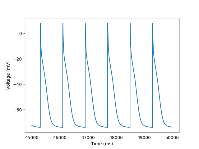
plt.figure()
plt.plot('t', 'vOld', data=trace)
plt.xlabel('Time (ms)')
_ = plt.ylabel('Voltage (mV)')

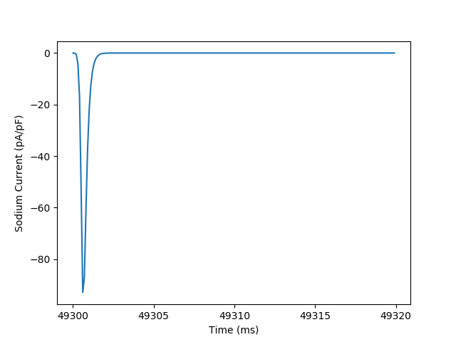
Using the saved data we can plot the traces for the variables we selected. We can also modify the data for analysis or to produce different plots as seen below for iNa where we subset the data to only plot the last sodium current peak.

trace_subset = trace[(trace['t'] > 49_300) & (trace['t'] < 49_320)]

plt.figure()
plt.plot('t', 'iNa', data=trace_subset)
plt.ylabel('Sodium Current (pA/pF)')
plt.xlabel('Time (ms)')
_ = plt.locator_params(axis='x', nbins=5)

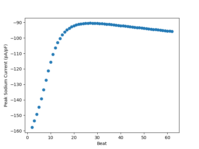
We can make a plots from the measured variables, such as seeing how the peak sodium current varies beat to beat throughout the simulation.

First we will enumerate the beats starting with 2 as we skipped the first beat using proto.meastime, then we will plot the beat vs peak sodium current, which in this case is captured by the min measure as sodium current is always negative

beat = np.arange(meas.shape[0])+2

plt.figure('Peak Sodium Current vs Beat')
plt.scatter(beat, meas[('iNa', 'min')])
plt.ylabel('Peak Sodium Current (pA/pF)')
_ = plt.xlabel('Beat')